Spam Email Detection using Machine Learning Projects for Beginners in Python (2023)

Topic – spam email detection using machine learning | Source Code |2023| GitHub (Thanks for making Live Color Detector in Python VIRAL)

Introduction

In this era of technology, the Internet has become a part of our daily life. Be it checking important emails, or be it commenting on your friend’s recent upload on Instagram or just reading customer reviews of a product you want to purchase through Amazon, any of these would have been impossible without the Internet.

But, wait.

Every coin has two sides, right?

This ultimate source of gathering information worldwide has also some unethical sides. To spell it more precisely, it is Internet Spam.

MUST-READ: Hands-on Exploratory Data Analysis Python Code & Steps  | MOST POPULAR PYTHON PROJECT

Internet Spam is a collection of irrelevant texts sent in the form of messages or emails, with the motive of promoting stuff, advertisements of websites that support online dating, pornography, and also phishing and spreading viruses.

This spam, if accidentally or intentionally clicked by you, can lead to your system being damaged by virus attacks, a waste of your network resources, and also a waste of time.

Well. That doesn’t sound good to the ears!

Technologies like Natural Language Processing, which is a major subfield of Artificial Intelligence, come here to play the game!

NLP deals with analyzing, extracting, and retrieving valuable information from text data for gathering human-like language insights for a wide range of applications like Spam Detection, Sentiment Analysis, language translations, and document classification.

Also, Check – MOST POPULAR PYTHON PROJECT |  Customer Churn Prediction using Machine Learning

Use Case of spam email detection using machine learning

In this article, we will understand how to implement and build a deep-learning model for Spam Detection. The model we will try to implement will be a Classifier, which would give binary outputs- either spam or ham.

Prerequisites–

Before starting with the next step, you must have a good understanding of deep learning algorithms, Dense Sequential Classifier Networks, Long-Short-Term-Memory Networks (LSTM), and Bidirectional LSTM (Bi-LSTM).

And, those who already have a good grasp of these algorithms, just skip this part jump to the next section, and start your setup required for this project!

Let’s begin with the setup and installation for spam email detection using machine learning

Will you be rich & famous ? Click Here to Find Out in 60 Seconds | Click Here

Setup and Installation–

• Programming Language – Python (>= 3x)
• External libraries for reading and exploring data – NumPy, Pandas, Seaborn, Matplotlib, word cloud
• Library for splitting data – Sklearn
• Library for deep learning – TensorFlow (>=2.0) as it contains Keras API

Note – If you work with any other versions of the required software libraries, make sure to create a separate virtual environment for the spam email detection project and install all the dependencies as said.

• Expert’s Advice On How Long It Takes to Learn Coding – READ NOW!
• Can a software developer become a billionaire? – WENT VIRAL !!

Data –

We will use the text data from UCI Datasets for the spam email detection project. This data contains 5.57k spam messages, which are labeled as spam or ham (not spam). We will use this data to train and test our model, by splitting it into train and test sub-datasets.

Note – Make sure to keep all datasets in the same directory where your project source code is located, otherwise you will get an error, as your path cannot be detected.

Problem-Solving Approach–

We will implement a Dense Classifier Sequential Neural Network, the next one with LSTM, and further with Bi-LSTM, and compare our accuracies and results in the end to select the best one!

Steps to cover-up –

1. Import dependencies; load and analyze the spam text data
2. Split the data into train and test sub-datasets; text preprocessing
3. Train our model using the three deep-learning algorithms
4. Compare results and select the best model
5. Use the final classifier to detect spam messages

So, let us see who wins the game, Dense Sequential, LSTM, or Bi-LSTM! 😎

Step 1: Import dependencies; load and analyze the spam text data

Let us import all the required packages, at once.

# import libraries for reading data, exploring and plotting
import numpy as np
import pandas as pd
import seaborn as sns
import matplotlib.pyplot as plt
from wordcloud import WordCloud, STOPWORDS, ImageColorGenerator

%matplotlib inline

# library for train test split
from sklearn.model_selection import train_test_split

# deep learning libraries for text pre-processing
import tensorflow as tf
from tensorflow.keras.preprocessing.text import Tokenizer
from tensorflow.keras.preprocessing.sequence import pad_sequences

# Modeling 
from tensorflow.keras.callbacks import EarlyStopping
from tensorflow.keras.models import Sequential
from tensorflow.keras.layers import Embedding, GlobalAveragePooling1D, Dense, Dropout, LSTM, Bidirectional

Let’s load and explore the data now!

path = '/content/drive/MyDrive/spam/SMSSpamCollection'
messages = pd.read_csv(path, sep ='\t',names=["label", "message"])
messages[:3]

We will get the 1st three rows of our dataset in the output, which will ensure that we have properly loaded our data!

Let us get into some statistical analysis and visualize the data.

We will get short summary details of our data with the .describe() function.

messages.describe()

Let’s look at the output.

The output shows that our message count is 5572, where 2 unique labels are “spam” and “ham” , and the unique message count is 5169, as the rest are repeated ones. The top label is ‘ham’ and the top message is ‘Sorry, I’ll call later.

Since there are duplicate messages, let’s store them on a separate variable ‘duplicatedRow’ and check if it’s properly filtered out.

MUST READ – How to Get a Coding Job with No Experience [Updated]

duplicatedRow = messages[messages.duplicated()]
print(duplicatedRow[:5])

Look at the output. It successfully printed the results.

Now, let us get some summary statistics by labels.

messages.groupby('label').describe().T

Let us see what this summary tells us-

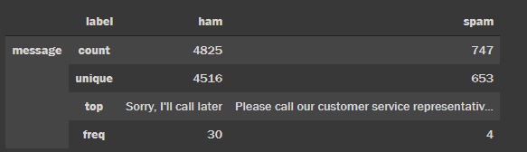
There are 4,825 ham and 747 spam messages. This indicates the data is imbalanced which needs to be fixed.

The top ham message is “Sorry, I’ll call later”, whereas the top spam message is “Please call our customer service…” which occurred 30 and 4 times, respectively.

First, let’s create a separate data frame for ham and spam messages and convert it to a NumPy array and then to a list to generate WordCloud later.

# Get all the ham and spam messages
ham_msg = messages[messages.label =='ham']
spam_msg = messages[messages.label=='spam']

# Create numpy list to visualize using wordcloud
ham_msg_txt = " ".join(ham_msg.message.to_numpy().tolist())
spam_msg_txt = " ".join(spam_msg.message.to_numpy().tolist())

Since it is text data, there are many unnecessary stopwords like articles, prepositions, etc., which need to be removed from the data.

So, let us create our word cloud now, to extract the most frequent words in ham messages.

# wordcloud of ham messages
ham_msg_wcloud = WordCloud(width =520, height =260, stopwords=STOPWORDS,max_font_size=50, background_color ="red", colormap='Blues').generate(ham_msg_txt)
plt.figure(figsize=(16,10))
plt.imshow(ham_msg_wcloud, interpolation='bilinear')
plt.axis('off') # turn off axis
plt.show()

And this generates a cool WordCloud!

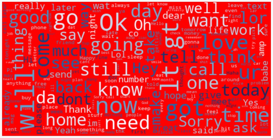
The ham message WordCloud above shows that “love”, “will”, “come”, “now” and “time” are the most commonly appeared word in ham messages.

Let us do the same for spam messages and see what it shows!

# wordcloud of spam messages
spam_msg_wcloud = WordCloud(width =520, height =260, stopwords=STOPWORDS,max_font_size=50, background_color ="black", colormap='Spectral_r').generate(spam_msg_txt)
plt.figure(figsize=(16,10))
plt.imshow(spam_msg_wcloud, interpolation='bilinear')
plt.axis('off') # turn off axis
plt.show()

Let us look at the WordCloud generated!

The spam message WordCloud above shows that “FREE”, “call”, “text”, “GUARANTEED” and“win” are the most commonly appeared words in spam messages.

Awesome!

Now, since our data is imbalanced, we need to plot a bar graph to estimate the percentage of spam and ham ratio.

#visualize imbalanced data 
plt.figure(figsize=(8,6))
sns.countplot(messages.label)
# Percentage of spam messages
(len(spam_msg)/len(ham_msg))*100 

Look at the output bar graph generated.

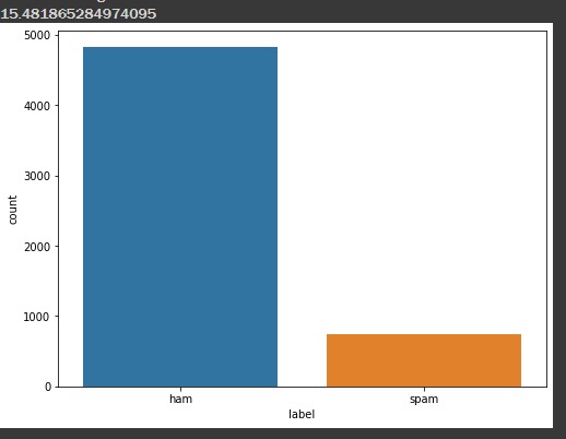
So, it clearly shows that the percentage of spam messages is approximately 15.48%. So we can estimate that the percentage of ham and spam is 85% and 15% respectively.

Next, we have to deal with our imbalanced data issue. There are several techniques to fix imbalanced data. For our use case, we will be using the Downsampling method.

In downsampling, we delete some records from the majority class of the data (ham here), so that it matches the minority class count (spam here). Hence, our data will no longer be imbalanced, and it won’t misclassify the messages.

So, let us implement a downsampling method for our imbalanced data!

# one way to fix imbalanced data is to downsample the ham message count to the spam message count
ham_msg_df = ham_msg.sample(n = len(spam_msg), random_state = 44)
spam_msg_df = spam_msg

#check the shape now, it must be te same!
print(ham_msg_df.shape, spam_msg_df.shape)

#check graph for better visualization 
msg_df = ham_msg_df.append(spam_msg_df).reset_index(drop=True)
plt.figure(figsize=(8,6))
sns.countplot(msg_df.label)
plt.title('Distribution of ham and spam messages (after downsampling)')
plt.xlabel('Message labels')

Now, look at the output! Both spam and ham counts are the same.

(747, 2) (747, 2)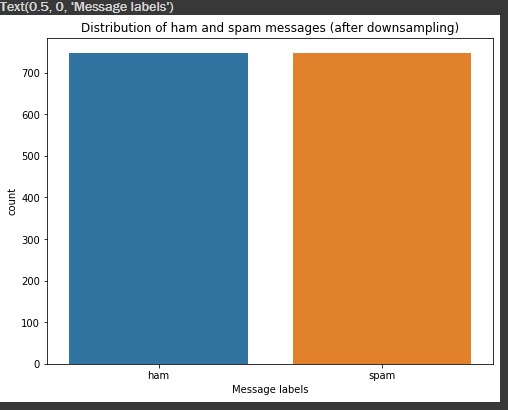

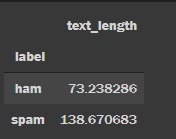
Now, let us compute the text length of spam and ham messages, which we will need later.

# Get length column for each text
msg_df['text_length'] = msg_df['message'].apply(len)

#Calculate average length by label types
labels = msg_df.groupby('label').mean()
labels

This will output us a table containing, text lengths of spam and ham messages.

Step 2: Split the data into train and test sub-datasets; text preprocessing

Let’s convert our categorical labels to numerical labels, i.e. 0 for ham and 1 for spam. Then we will split our data into train and test sets. Further, we will transform the labels to numpy arrays, for fitting our models.

Note – Train and Test data should have a ratio of 8:2 (80% training data and 20% test data).

# Map ham label as 0 and spam as 1
msg_df['msg_type']= msg_df['label'].map({'ham': 0, 'spam': 1})
msg_label = msg_df['msg_type'].values

# Split data into train and test
train_msg, test_msg, train_labels, test_labels = train_test_split(msg_df['message'], msg_label, test_size=0.2, random_state=434)

Run this, and let us get our hands on text preprocessing, which is one of the most crucial steps to perform before modeling.

To preprocess your text is equivalent to making your text suitable for analysis, modeling, and prediction. It is done by Tokenization, Sequencing, and Padding techniques.

Firstly, we will tune the hyper-parameters used for preprocessing.

# Defining pre-processing hyperparameters
max_len = 50 
trunc_type = "post" 
padding_type = "post" 
oov_tok = "<OOV>" 
vocab_size = 500

We will now use Tokenizer() to tokenize the words into a numerical representation. We will be using the Tokenizer API from TensorFlow Keras. It splits up sentences into words and performs integer encoding.

tokenizer = Tokenizer(num_words = vocab_size, char_level=False, oov_token = oov_tok)
tokenizer.fit_on_texts(train_msg)

We can get the word_index by using tokenizer.word_index.

# Get the word_index 
word_index = tokenizer.word_index
word_index

Let us look at the word indexes it printed.

Now let us see how many unique tokens are there in our data.

# check how many unique tokens are present
tot_words = len(word_index)
print('There are %s unique tokens in training data. ' % tot_words)

Output-

There are 4169 unique tokens in training data. 

Now let us begin the next preprocessing task- Sequencing and Padding.

Sequencing will represent each sentence by sequences of numbers using texts_to_sequences() from the tokenizer object. Next, we will use pad_sequences() so that each sequence will have the same length.

# Sequencing and padding 
#train
training_sequences = tokenizer.texts_to_sequences(train_msg)
training_padded = pad_sequences (training_sequences, maxlen = max_len, padding = padding_type, truncating = trunc_type )

#test
testing_sequences = tokenizer.texts_to_sequences(test_msg)
testing_padded = pad_sequences(testing_sequences, maxlen = max_len,padding = padding_type, truncating = trunc_type)

Great!

Our data is now preprocessed, and we can start training our models now.

Step 3: Train our model using the three deep-learning algorithms

Let us now use the three neural network architectures, mentioned earlier, for text classification.

The Dense Sequential Spam Detection Model–

Before coding the model architecture, let us quickly tune the hyperparameters.

vocab_size = 500 
embeding_dim = 16
drop_value = 0.2 
n_dense = 24

Let us design the model architecture now.

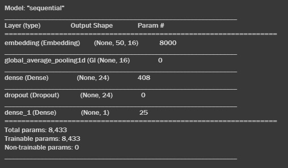
#Dense Sequential model architecture
model = Sequential()
model.add(Embedding(vocab_size, embeding_dim, input_length=max_len))
model.add(GlobalAveragePooling1D())
model.add(Dense(24, activation='relu'))
model.add(Dropout(drop_value))
model.add(Dense(1, activation='sigmoid'))

• Sequential – This is the Keras Sequential model. It has 3 layers- Embedding Layer, Pooling Layer, and Dense Layer.
• Embedding Layer – The 1st hidden layer of the network. Maps each token to an N-dimensional vector, making a sense that two words with similar meanings tend to have very close vectors.
• Pooling Layer – Converts layer to one dimension by reducing the number of parameters in the model hence helping to avoid overfitting.
• Dense Layer – The final layer that sends the output from the neural network. It has an activation function ‘relu’ followed by a dropout layer to avoid overfitting and a final output layer with a sigmoid activation function. The sigmoid activation function outputs probabilities between 0(ham) and 1(spam).

Let us look at the model summary.

model.summary()

Running this will output the entire summary of the model.

Let us compile the model now!

model.compile(loss='binary_crossentropy',optimizer='adam' ,metrics=['accuracy'])

• ‘binary_crossentropy’ – loss function for binary classification.
• ‘Adam’ – optimizer that uses momentum to avoid local minima
• ‘accuracy’ – a measure of model performance

Our model is now compiled and ready to be fitted to the training data.

Let’s fit the model.

# fit dense seq model
num_epochs = 30
early_stop = EarlyStopping(monitor='val_loss', patience=3)
history = model.fit(training_padded, train_labels, epochs=num_epochs, validation_data=(testing_padded, test_labels),callbacks =[early_stop], verbose=2)

• num_epochs – Iteration count of the learning algorithm through the entire training data set. 
• early_stop and callbacks – Callbacks allow you to specify the performance measure to monitor the trigger, and once triggered, it will stop the training process.
• verbose –  prints loss and accuracy on each epoch.

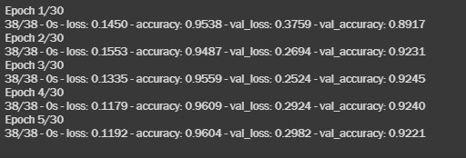
Let us look at the training process executed.

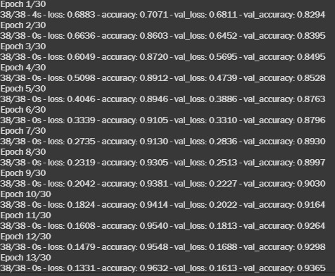
The model results we got after the 30th epoch, are as follows-

• training loss: 0.05
• training accuracy: 98%
• validation loss: 0.11
• validation accuracy: 94.6% ~ 95%

That’s pretty great!

Let us test this awesome learning on test data and see how the model predicts unknown labels.

# Model performance on test data 
model.evaluate(testing_padded, test_labels)

Let us look at the results-

The results are as follows-

• loss – 0.11
• accuracy – 94.65

We will now visualize the historical results by plotting loss and accuracy Vs. number of epochs.

metrics = pd.DataFrame(history.history)
# Rename column
metrics.rename(columns = {'loss': 'Training_Loss', 'accuracy': 'Training_Accuracy', 'val_loss': 'Validation_Loss', 'val_accuracy': 'Validation_Accuracy'}, inplace = True)
def plot_graphs1(var1, var2, string):
    metrics[[var1, var2]].plot()
    plt.title('Training and Validation ' + string)
    plt.xlabel ('Number of epochs')
    plt.ylabel(string)
    plt.legend([var1, var2])
plot_graphs1('Training_Loss', 'Validation_Loss', 'loss')

Let us visualize the output generated.

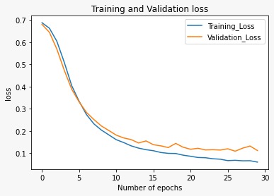
The plot above shows, that the accuracy is increasing over increasing epochs. As expected, the model is performing better in the training set than in the validation set.

Great job indeed!

The LSTM spam detection model:

Let’s fit the spam detection model using LSTM. First, let’s tune our hyperparameters. Then we will code the model architecture.

#LSTM hyperparameters
n_lstm = 20
drop_lstm =0.2

• n_lstm – the number of nodes in the hidden layers within the LSTM cell
• drop_lstm – a dropout, that prevents overfitting

#LSTM Spam detection architecture
model1 = Sequential()
model1.add(Embedding(vocab_size, embeding_dim, input_length=max_len))
model1.add(LSTM(n_lstm, dropout=drop_lstm, return_sequences=True))
model1.add(LSTM(n_lstm, dropout=drop_lstm, return_sequences=True))
model1.add(Dense(1, activation='sigmoid'))

Now, we will compile our model.

model1.compile(loss = 'binary_crossentropy', optimizer = 'adam', metrics=['accuracy'])

Let us train our model!

num_epochs = 30
early_stop = EarlyStopping(monitor='val_loss', patience=2)
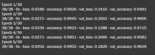
history = model1.fit(training_padded, train_labels, epochs=num_epochs, validation_data=(testing_padded, test_labels),callbacks =[early_stop], verbose=2)

Let us look at the training process executed.

The results are as follows-

• loss: 0.1192
• accuracy: 0.9604
• validation loss: 0.2982
• validation accuracy: 0.9221

Let us plot training Vs. validation loss.

metrics = pd.DataFrame(history.history)
# Rename column
metrics.rename(columns = {'loss': 'Training_Loss', 'accuracy': 'Training_Accuracy',
                         'val_loss': 'Validation_Loss', 'val_accuracy': 'Validation_Accuracy'}, inplace = True)
def plot_graphs1(var1, var2, string):
    metrics[[var1, var2]].plot()
    plt.title('LSTM Model: Training and Validation ' + string)
    plt.xlabel ('Number of epochs')
    plt.ylabel(string)
    plt.legend([var1, var2])
plot_graphs1('Training_Loss', 'Validation_Loss', 'loss')

Let us visualize the graph generated.

The results are somewhat positive, but somewhere in between the training, the loss is increasing, which leads to lesser accuracy than the Dense Sequential Model.

Bi-directional Long Short Term Memory (BiLSTM) Model:

Bi-LSTM is a smart guy and looks both forward and backward while crossing the street! It learns patterns from both before and after a given token within a text. The Bi-LSTM back-propagates in both backward and forward directions in time.

The computational time is more compared to LSTM. But, in most cases, Bi-LSTM results in better accuracy.

The hyperparameters are the same as LSTM. So, we can code the architecture!

# Biderectional LSTM Spam detection architecture
model2 = Sequential()
model2.add(Embedding(vocab_size, embeding_dim, input_length=max_len))
model2.add(Bidirectional(LSTM(n_lstm, dropout=drop_lstm, return_sequences=True)))
model2.add(Dense(1, activation='sigmoid'))

Compile, compile, compile!

model2.compile(loss = 'binary_crossentropy', optimizer = 'adam', metrics=['accuracy'])

Let’s train this smart kid.

# Training
num_epochs = 30
early_stop = EarlyStopping(monitor='val_loss', patience=2)
history = model2.fit(training_padded, train_labels, epochs=num_epochs, 
                    validation_data=(testing_padded, test_labels),callbacks =[early_stop], verbose=2)

Let us look at the training results.

The results are as follows-

• loss: 0.0254
• accuracy: 0.9952
• validation loss: 0.1826
• validation accuracy: 0.9629

Uh, oh! That is close to Dense!

Let us visualize the training Vs. Validation loss.

metrics = pd.DataFrame(history.history)
# Rename column
metrics.rename(columns = {'loss': 'Training_Loss', 'accuracy': 'Training_Accuracy',
                         'val_loss': 'Validation_Loss', 'val_accuracy': 'Validation_Accuracy'}, inplace = True)
def plot_graphs1(var1, var2, string):
    metrics[[var1, var2]].plot()
    plt.title('BiLSTM Model: Training and Validation ' + string)
    plt.xlabel ('Number of epochs')
    plt.ylabel(string)
    plt.legend([var1, var2])
# Plot
plot_graphs1('Training_Loss', 'Validation_Loss', 'loss')

And, here is our graph.

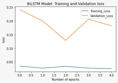
Though the validation loss decreased at the beginning, it again stepped up at the end. It is not as smooth as Dense, but a little better than LSTM.

Step 3 was quite fun! Now let’s quickly compare the 3 models.

Step 4: Compare results and select the best model

This simple code will compare the 3 models, all at once.

# Comparing three different models
print(f"Dense architecture loss and accuracy: {model.evaluate(testing_padded, test_labels)} " )
print(f"LSTM architecture loss and accuracy: {model1.evaluate(testing_padded, test_labels)} " )
print(f"Bi-LSTM architecture loss and accuracy: {model2.evaluate(testing_padded, test_labels)} " )

Look at the output-

Among all, both Dense and BiLSTM outperformed the LSTM. Based on loss, accuracy, and the plots above, we select Dense architecture as a final model for classifying text messages as spam or ham.

Seems like Dense won the match! 😎

Step 5: Use the final classifier to detect spam messages

Let’s evaluate how our Dense spam detection model predicts/classifies whether it is spam or ham given the text from our original data.

predict_msg = ["Go until jurong point, crazy.. Available only in bugis n great world la e buffet... Cine there got amore wat...",
          "Ok lar... Joking wif u oni...",
          "Free entry in 2 a wkly comp to win FA Cup final tkts 21st May 2005. Text FA to 87121 to receive entry question(std txt rate)T&C's apply 08452810075over18's"]
# Defining prediction function
def predict_spam(predict_msg):
    new_seq = tokenizer.texts_to_sequences(predict_msg)
    padded = pad_sequences(new_seq, maxlen =max_len,
                      padding = padding_type,
                      truncating=trunc_type)
    return (model.predict(padded))
predict_spam(predict_msg)

You will be amazed after getting the output!

As you can see, the array displayed predicts that there is a 99% chance for the 3rd message to be spam.

And it’s absolutely correct!

By Author,

Hope you had a good hands-on with spam email detection using machine learning and learned a lot about spam detection with deep learning!

This article provides an overview of using different architectural deep learning models for NLP problems using TensorFlow2 Keras.

You can view my notebook and download data from my GitHub.

Thank you and do give a try to spam email detection using machine learning!

Feel free to discuss further and connect with me on LinkedIn, GitHub, and Medium. Stay tuned with the programming projects category to find more amazing ML/AI/Python projects

This concludes the topic of spam email detection using machine learning (Best machine learning projects for beginners in Python) To know more about such topics go through My Blind Bird.

You can check out our other projects with source code below-

1. Fake News Classifier with NLP 2023
2. Hands-on Exploratory Data Analysis Python Code & Steps -2023
3. Interesting Python project (2023) Mouse control with hand gestures.
4. Best (2023) Python Project with Source Code
5. Live Color Detector (#1 ) in Python 2023
6. Projects for beginners in Python

Happy Learning!

September 27, 2023